How To Draw Root Locus In Matlab

Introduction to Root Locus Matlab

The Due west.R. Evans developed the root locus method. It is widely used in control applied science for the design and analysis of control systems. In this method, organization poles are plotted against the value of a system parameter, especially the open up-loop transfer office proceeds root locus analysis is a graphical method for examining how the roots of a system change with variation of a certain organization parameter are typically used in control theory and stability theory. In this topic, we are going to learn about Root Locus Matlab.

Syntax

The syntax for Root Locus Matlab is every bit shown below:-

rlocus (sys)

How to Do Root Locusmatlab?

In a Matlab for a root locus, rlocus inbuilt function is available. For using these inbuilt rlocus function, we need to create one transfer function on a Matlab; for that, nosotros can apply a tf inbuilt office which can be available on Matlab.

Let us encounter how we used these function to brandish the root locus. For that, first, we demand to create i transfer function. For creating a transfer function, we need to know the coefficients of the numerator and denominator of that transfer function

we create transfer function in two ways. The ways are as follows:-

1. Num3= [25 ];

Den3 = [ane -1 -two];

TF1 = tf (Num3 , Den3)

In a first way, nosotros can take two variables to shop the numerator and denominator coefficients and and then we just pass those two variables on tf office and that a comma separates two variables.

2. GH1 = tf([1],[1 five half-dozen 0])

In the tf role, we take ii foursquare brackets; in the start foursquare brackets, we write the coefficients of the numerator (club s^four, south^three……, due south, constant), and in 2d square brackets, we write coefficients of the denominator (order due south^4, s^iii……, s, constant). The comma separates these two square brackets.

And then use rlocus function in brackets the variable which is assigned for the transfer function.

Examples of Root Locus Matlab

Here are the following examples mention below

Example ane

Let us consider one example,

In this instance, we have one transfer function for that we create 2 variables, 'num1' and 'den1', respectively. The variable 'num1' contains the coefficients of the numerator of the transfer office, and variable 'den1' stores the coefficients of the denominator of the transfer role. The tf part generates a transfer office for given coefficients of 'num1' and 'den1' variables on Matlab. Then using two variables of transfer function 'num1' and 'den1', we can display the transfer function and stored it in variable 'TF1'.Then utilize the 'rlocus' role in brackets the variable which is assigned for transfer part 'TF1'.

Code:

clc;
clear all;
close all;
num1= [one iii ];
den1 = [1 -1 -ii];
disp ('Transfer function :-  ');
TF1 = tf (num1 , den1)
rlocus(TF1)

Output:

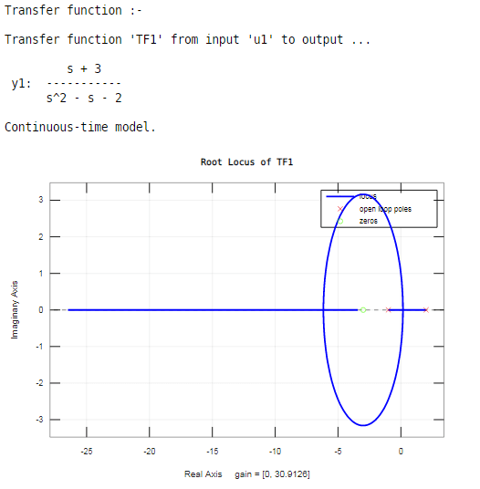
As shown in the resultant rot locus, information technology can bear witness poles and zeros. For locating poles, the '×' sign is used, and for zeros, the 'o' sign is used on a root locus.

Root locus exists on the real axis between:
ii and -1
-iii and negative infinity

Instance 2

Let u.s.a. see ane more instance related to root locus Matlab,

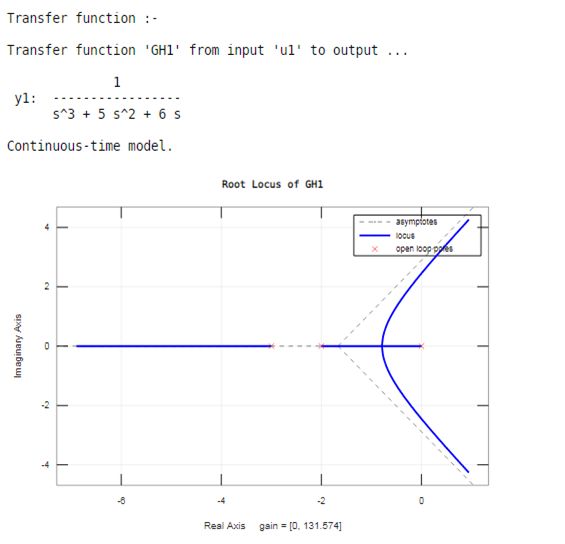
In this example, we tin accept the above transfer role for a root locus. Nosotros create the above transfer function on Matlab by using the tf inbuilt office. In tf part, nosotros assign the coefficients of the in a higher place transfer function; in tf function, we take two square brackets, in first foursquare brackets, we write the coefficients of numerator for the above transfer function (order s^4, s^3, ……, south, constant) and in second foursquare brackets, nosotros write coefficients of the denominator for higher up transfer part (order s^4, s^three……, due south, constant). The comma separates these ii square brackets. And then we utilise a rlocus function in brackets; we assign the variable which is use to generate a transfer part.

Code:

clc;
clear all;
close all;
disp ('Transfer function :-  ');
GH1 = tf ( [ i ] , [ one v 6 0 ] )
rlocus (GH1)

Output:

Case #3

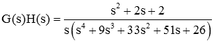
Let us consider another 1 example,

Code:

clc;
clear all;
shut all;
disp ('Transfer office :-  ');
sys = tf ( [ one ii 3 ] , [ 1 ix 34 51 2810 ] )
rlocus(sys)

Output:

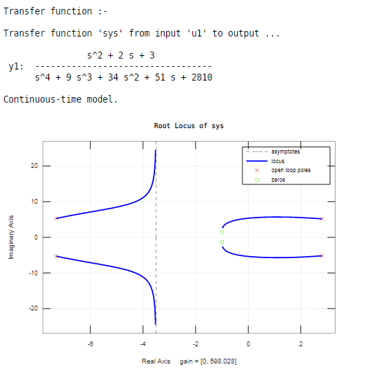
In this example, we accept five poles and two zeros. The poles are shown by '×', and the zeros are shown by 'o' on a root locus.

Root locus exists on the real axis betwixt:
0 and -1
-ii and negative infinity

Recommended Articles

This is a guide to Root Locus Matlab. Here we discuss the basic concepts of root locus. And how we employ a root locus in Matlab, what exactly syntax is used to create a root locus. In this article, we also saw some examples related to root locus with Matlab codes. You may also have a look at the post-obit articles to learn more –

1. Matlab Syms
2. Matlab Format
3. Dot Product MATLAB
4. Moving Average Matlab

Source: https://www.educba.com/root-locus-matlab/

Posted by: khangwartan.blogspot.com

Share this post